Fully Periodic Double Shear Layer

View on GitLab

Inspired by [15].

Domain Setup and Initial State

The double shear-layer problem runs on a (pseudo-)two-dimensional fully periodic domain of $N \times N$ cells. The physical domain size is normalized to the unit square ($[0, 1]^2$), such that the cell spacing in x- and y-direction is $h = \frac{1}{N}$.

The density and velocity fields are initialized to the following state, depending to the initial velocity magnitude $u_0$, shear layer width $\kappa$ and vertical perturbation $\delta$:

\begin{align} \rho(x, y) &= 1 \\ u_x (x, y) &= \begin{cases} u_0 \tanh{ \left( \kappa (y - \frac{1}{4}) \right) } & \text{if } y \le \frac{1}{2} \\ u_0 \tanh{ \left( \kappa (\frac{3}{4} - y) \right) } & \text{if } y > \frac{1}{2} \end{cases} \\ u_y (x, y) &= \delta u_0 \sin{ \left( 2 \pi \left( x + \frac{1}{4} \right) \right) } \end{align}

This example showcases a portable parallel simulation app built with waLBerla V8, solving the transient evolution from the above initial conditions.

Code Generation

The numerical kernels for the double shear-layer application are generated by the script DoubleShearLayerSweeps.py.

Preamble

The preamble of the scripts imports all required functions and classes from the pycodegen packages and SweepGen:

from lbmpy import (
    LBStencil,
    Stencil,
    LBMConfig,
    Method,
)
 
import sympy as sp
import pystencils as ps
 
from pystencilssfg import SourceFileGenerator
import sweepgen as sg
from sweepgen.build_config import DEBUG
from sweepgen.symbolic import cell
from sweepgen.prefabs import LbmBulk

Next, we open the code generation manager, enable the walberla::v8 field classes, and set the namespace:

with SourceFileGenerator() as sfg:
    sg.Sweep.use_v8core_fields()
    sfg.namespace("DoubleShearLayer::gen")

Numerical Kernels

The application will comprise three numerical components:

• The lattice Boltzmann bulk dynamics, including PDF initialization and the stream-collide-sweep;
• Setup of the initial state of the density and velocity fields;
• Computation of the vorticity from the velocity field during post-processing.

LBM Bulk Dynamics

We start by defining the lattice Boltzmann method using lbmpy's configuration API. We pass this to the LbmBulk prefab to generate the sweeps for the bulk dynamics:

    stencil = LBStencil(Stencil.D3Q19)
    lbm_config = LBMConfig(
        stencil=stencil,
        method=Method.SRT,
        compressible=True,
        relaxation_rate=sp.Symbol("omega"),
    )
 
    lbm_bulk = LbmBulk(sfg, "LBM", lbm_config)
    sfg.generate(lbm_bulk)

Initial State

Then, we encode the above equations defining the initial state using SymPy and pystencils.flow, and produce an initialization sweep from them:

    rho, u = lbm_bulk.rho, lbm_bulk.u
 
    #   Initial State
 
    @sg.flow.generate_sweep(sfg)
    def SetInitialState(_eq):
        u_0, kappa, delta = sp.symbols("u_0, kappa, delta")
 
        _eq.store[rho()] = 1
 
        _eq.store[u(0)] = sp.Piecewise(
            (
                u_0 * sp.tanh(kappa * (cell.y() - sp.Rational(1, 4))),
                cell.y() <= sp.Rational(1, 2),
            ),
            (
                u_0 * sp.tanh(kappa * (sp.Rational(3, 4) - cell.y())),
                cell.y() > sp.Rational(1, 2),
            ),
        )
 
        _eq.store[u(1)] = (
            delta * u_0 * sp.sin(2 * sp.pi * (cell.x() + sp.Rational(1, 4)))
        )
        _eq.store[u(2)] = 0
 
    #   end initial state

Finite Differences for Vorticity

Finally, we set up a sweep computing the 2D vorticity from the velocity field using finite differences:

    #   Compute Vorticity
 
    @sg.flow.generate_sweep(sfg)
    def ComputeVorticity(_eq):
        dvx, duy = sp.symbols("dvx, duy")
        vorticity = ps.fields(f"vorticity: double[{stencil.D}D]", layout="fzyx")
 
        _eq.let[dvx] = (u[1, 0, 0](1) - u[-1, 0, 0](1)) / (2 * cell.dx())
        _eq.let[duy] = (u[0, 1, 0](0) - u[0, -1, 0](0)) / (2 * cell.dy())
        _eq.store[vorticity()] = (dvx - duy) / 2
 
    #   end vorticity

Application Frame

The C++ simulation application is implemented in DoubleShearLayer.cpp.

Preamble

The application code begins with the inclusion of all required header files, and namespace declarations:

#include "blockforest/all.h"
 
#include "core/all.h"
 
#include "domain_decomposition/SharedSweep.h"
 
#include "stencil/all.h"
 
#include "timeloop/all.h"
 
#include "vtk/all.h"
 
#include "gen/DoubleShearLayerSweeps.hpp"
#include "walberla/v8/HaloExchange.hpp"
#include "walberla/v8/Memory.hpp"
#include "walberla/v8/Sweep.hpp"
 
namespace DoubleShearLayer

Next, we define a few type aliases. We automatically select the memory tag from the build configuration; We set up field types for the scalar and vector fields, as well as the LBM Stencil and PDF field type. These must match the stencil used in the code generator script (see above) in both dimensionality and size of the velocity set.

using namespace walberla;
using namespace walberla::v8;
 
using MemoryTag = memtag::automatic;
 
using ScalarField_T = memory::Field< real_t, 1, MemoryTag >;
using VectorField_T = memory::Field< real_t, 3, MemoryTag >;
 
using LbStencil  = stencil::D3Q19;
using PdfField_T = memory::Field< real_t, LbStencil::Q, MemoryTag >;

Domain and Fields Setup

Next comes the primary workhorse: The run method. It starts off by taking the C command line arguments and forwarding them to the waLBerla environment singleton. Then, options controlling the domain setup are read from the parameter file and the simulation domain is initialized.

void run(int argc, char** argv)
{
   Environment env{ argc, argv };
   auto config = env.config();
 
   Config::BlockHandle domainParams = config->getBlock("Domain");
 
   Vector3< uint_t > numBlocks     = domainParams.getParameter< Vector3< uint_t > >("blocks");
   Vector3< uint_t > cellsPerBlock = domainParams.getParameter< Vector3< uint_t > >("cellsPerBlock");
 
   WALBERLA_CHECK_EQUAL(cellsPerBlock[0], cellsPerBlock[1], "Number of cells in x- and y- direction must be the same");
 
   AABB domainAabb{ 0., 0., 0., 1., 1., real_c(cellsPerBlock[2]) / real_c(cellsPerBlock[0]) };
   std::array< bool, 3 > periodic{ true, true, true };
 
   auto blocks = blockforest::createUniformBlockGrid(
      domainAabb, numBlocks[0], numBlocks[1], numBlocks[2], cellsPerBlock[0], cellsPerBlock[1], cellsPerBlock[2],
      /*oneBlockPerProcess*/ true, periodic[0], periodic[1], periodic[2]);
 

We then add the required fields to the domain:

   ScalarField_T rho{ *blocks };
   VectorField_T u{ *blocks };
   PdfField_T pdfs{ *blocks };
   ScalarField_T vorticity{ *blocks };

Parameters and Initial State

It is now time to set up the simulation's initial state, according to parameters provided by the user. These are the Reynolds number, the shear layer width and vertical perturbation, and the initial flow velocity. We read them from the parameter file and use them to set up and object of the initial-state sweep we generated above. We also set up the PDF initialization sweep from the LB bulk prefab. Then, we run both sweeps on all blocks of our simulation domain to prepare the fields:

   Config::BlockHandle simParams = config->getBlock("Parameters");
 
   const real_t reynolds{ simParams.getParameter< real_t >("Reynolds") };
   const real_t delta{ simParams.getParameter< real_t >("delta") };
   const real_t kappa{ simParams.getParameter< real_t >("kappa") };
   const real_t u_0{ simParams.getParameter< real_t >("u_0") };
 
   //  Initial State
 
   gen::SetInitialState setInitialState{ blocks, rho, u, delta, kappa, u_0 };
   gen::LBM::InitPdfs lbInit{ pdfs, rho, u };
 
   for (auto& b : *blocks)
   {
      setInitialState(&b);
      lbInit(&b);
   }

Simulation Loop

The main simulation loop comprises three parts: The LB stream-collide sweep, the vorticity computation, and the ghost layer synchronization. We set up the generated stream-collide sweep after computing the relaxation rate from the Reynolds number:

   //  Compute relaxation rate
   const real_t N = real_c(blocks->getDomainCellBB().xSize());
   const real_t nu{ (u_0 * N) / reynolds };
   const real_t theta{ 1_r / 3 };
   const real_t tau{ nu / theta };
   const real_t omega{ 2_r / (2_r * tau + 1_r) };
 
   auto streamCollide = std::make_shared< gen::LBM::StreamCollide >(pdfs, rho, u, omega);

Note

The stream-collide sweep uses the so-called pull streaming pattern, which requires a separate temporary array for memory safety. This array is managed internally by the sweep object. Due to this internal state, the stream-collide sweep is not copyable and must therefore be managed through a shared pointer.

Next, we prepare the communication scheme for ghost layer exchange. In addition to the pack info for the PDF field we also register a ghost-layer pack info for the velocity field. This is required by the finite-difference scheme of the vorticity sweep.

   //  Set up ghost layer communication
   auto haloExchange = HaloExchange::create< LbStencil, MemoryTag >(blocks)
                          .sendDirectlyFromGPU(false)
                          .sync(halo_exchange::streamPullSync< LbStencil >(pdfs))
                          .sync(u)
                          .makeShared();
 

Finally, we prepare the timeloop and register both sweeps and the communication scheme with it. Also, a time logger is created to print updates on the estimated runtime during the simulation:

   const uint_t numTimesteps{ simParams.getParameter< uint_t >("timesteps") };
   SweepTimeloop loop{ blocks->getBlockStorage(), numTimesteps };
 
   loop.add() << Sweep(makeSharedSweep(streamCollide)) << AfterFunction(SharedFunctor(haloExchange));
   loop.add() << Sweep(gen::ComputeVorticity{ blocks, u, vorticity });
 
   RemainingTimeLogger logger{ numTimesteps };
   loop.addFuncAfterTimeStep(logger);

VTK Output for Visualization

One last thing remains to be done before we can run the simulation: We need to export its results in the VTK format for later visualization using ParaView. If VTK is enabled, we create the VTK output object; and register output functions for the density, velocity, and vorticity fields with it; and add it to the time loop:

   Config::BlockHandle outputParams = config->getBlock("Output");
 
   const uint_t vtkWriteFrequency = outputParams.getParameter< uint_t >("vtkWriteFrequency", 0);
   if (vtkWriteFrequency > 0)
   {
      auto vtkOutput = vtk::createVTKOutput_BlockData(*blocks, "vtk", vtkWriteFrequency, 0, false, "vtk_out",
                                                      "simulation_step", false, true, true, false, 0);
 
      auto densityWriter = make_shared< memory::FieldVtkWriter< ScalarField_T, float32 > >(rho, "density");
      vtkOutput->addCellDataWriter(densityWriter);
 
      auto velWriter = make_shared< memory::FieldVtkWriter< VectorField_T, float32 > >(u, "velocity");
      vtkOutput->addCellDataWriter(velWriter);
 
      auto vorticityWriter = make_shared< memory::FieldVtkWriter< ScalarField_T, float32 > >(vorticity, "vorticity");
      vtkOutput->addCellDataWriter(vorticityWriter);
 
      loop.addFuncAfterTimeStep(vtk::writeFiles(vtkOutput), "VTK Output");
   }

Invoke the Timeloop

Lastly, the timeloop is invoked and the run-function ends:

   loop.run();
}
} // namespace DoubleShearLayer

Of course, the entire application must also have a main function, which is placed at the bottom of the file and invokes run:

int main(int argc, char** argv)
{
   DoubleShearLayer::run(argc, argv);
   return EXIT_SUCCESS;
}

CMake Target Definition

To build the app, we need to register it with CMake. In the beginning of our CMakeLists.txt, we first make sure to link any parameter files to the build directory:

walberla_link_files_to_builddir (*.prm)

We add an executable and register the application frame as a source file. For portability between CPU and GPU, we use walberla_set_gpu_language to set the correct GPU compilation language for our source files.

add_executable (DoubleShearLayer)
target_sources (DoubleShearLayer PRIVATE DoubleShearLayer.cpp)
walberla_set_gpu_language (DoubleShearLayer.cpp)

Then, we register the code generation script such that its output files will be linked against the application. We set the AUTO_LANGUAGE option such that the code generator selects the correct output language for the current GPU target:

walberla_generate_sources (DoubleShearLayer SCRIPTS DoubleShearLayerSweeps.py AUTO_LANGUAGE)

Finally, we need to link the app against waLBerla's runtime libraries:

target_link_libraries (
    DoubleShearLayer
    PRIVATE walberla::v8
)

Build and Run the App

Compilation

If not already done, generate the waLBerla build system with the V8 Core and SweepGen enabled by running this command in the waLBerla project root:

cmake -S . -B build -DWALBERLA_ENABLE_V8CORE=ON -DWALBERLA_ENABLE_SWEEPGEN=ON

Depending on your hardware, you may optionally enable OpenMP, CUDA or HIP for parallelization.

Navigate to build/apps/examples/DoubleShearLayer and build the app:

cd build/apps/examples/DoubleShearLayer
make -j

Parametrization and Execution

We use the following pre-defined parameter file (DoubleShearLayer.prm) to run the simulation:

Domain
{
    blocks < 1, 1, 1 >;
    cellsPerBlock < 256, 256, 8 >;
}
 
Parameters
{
    Reynolds 30000;
    kappa   80;
    u_0     0.04;
    delta   0.05;
 
    timesteps     7001;
}
 
Output
{
    vtkWriteFrequency   1000;
}

Start the simulation by calling ./DoubleShearLayer DoubleShearLayer.prm. Depending on your hardware, the simulation run can take several minutes. To review the results, open the file vtk_out/vtk.pvd in ParaView and investigate the velocity and vorticity arrays. Vorticity, when viewed from above, should look like this:

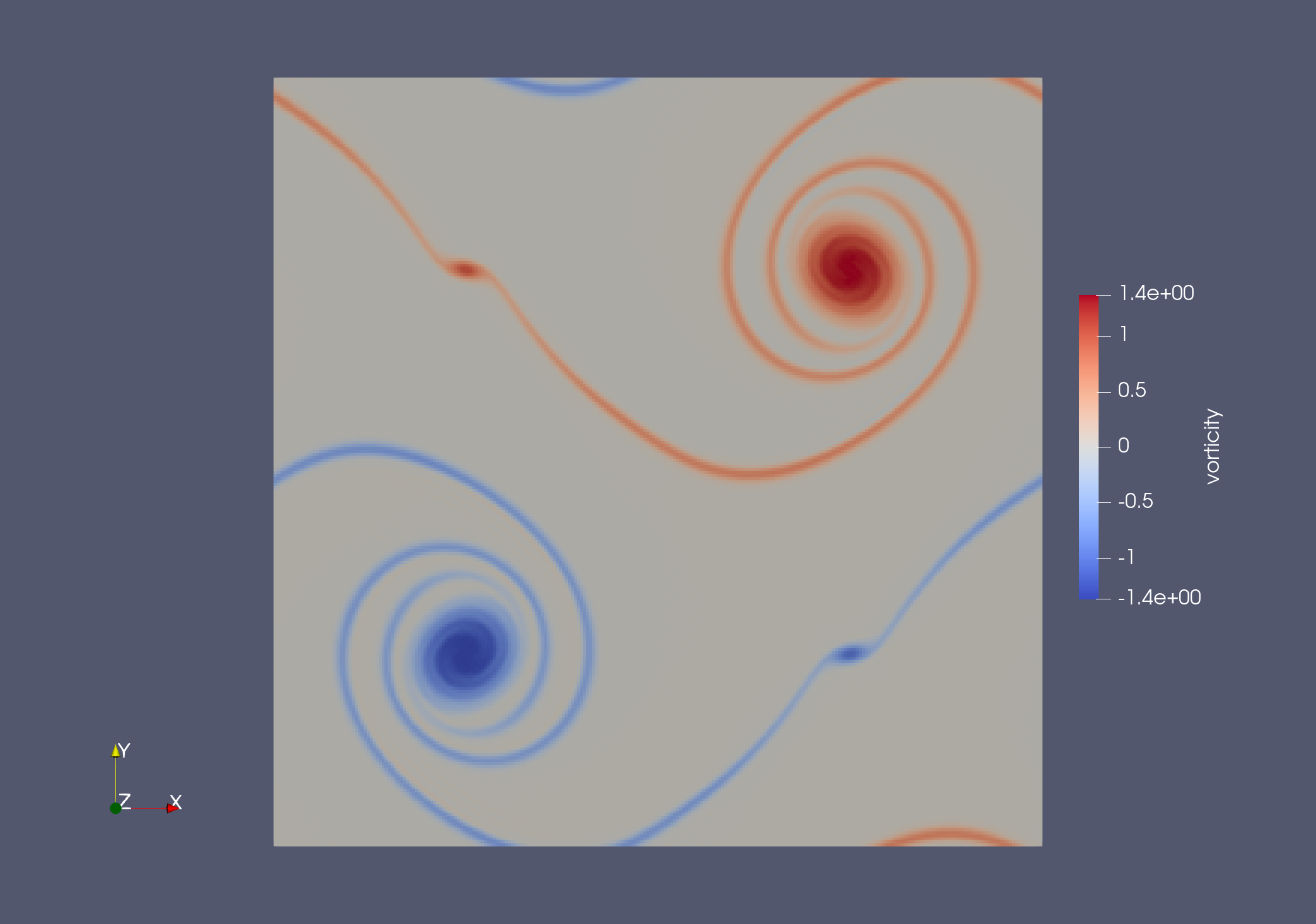
Plot of the Vorticity after 7000 time steps