Tutorial - LBM 4: Complex Geometry

Table of Contents

• Overview
• General Setup
• Lattice Boltzmann Data Structures
  • Lattice Model
  • Mesh and Domain
  • Boundary Handling
• Outlook

A configurable application for LBM simulations with complex geometries

NOTE: for this tutorial, you must have built waLBerla with WALBERLA_BUILD_WITH_OPENMESH enabled!

Overview

In this tutorial, the basic LBM setup from Tutorial LBM 1 is extended by the capability of handling complex geometries loaded from mesh files. It has following features:

• make use of default LBM sweeps from the lbm module
• can handle some basic boundary conditions: no slip, free slip, pressure, and velocity boundaries
• initialize geometry of the domain importing a mesh file (must be exported as triangle mesh in this tutorial)
• the boundary and geometry can be configured in a parameter file

The LBM routine mostly follows what has been demonstrated in LBM Tutorial 1. However, as our aim to load arbitrary complex geometry from a mesh file, we cannot specify the geometry via the Boundaries Block in the configuration file. We use waLBerla's mesh module that utilizes OpenMesh for loading, storing and manipulating meshes. Note that you must build waLBerla with OpenMesh capabilities in order to do this tutorial.

Stanford Bunny (loaded from an object file) in a 3D channel

General Setup

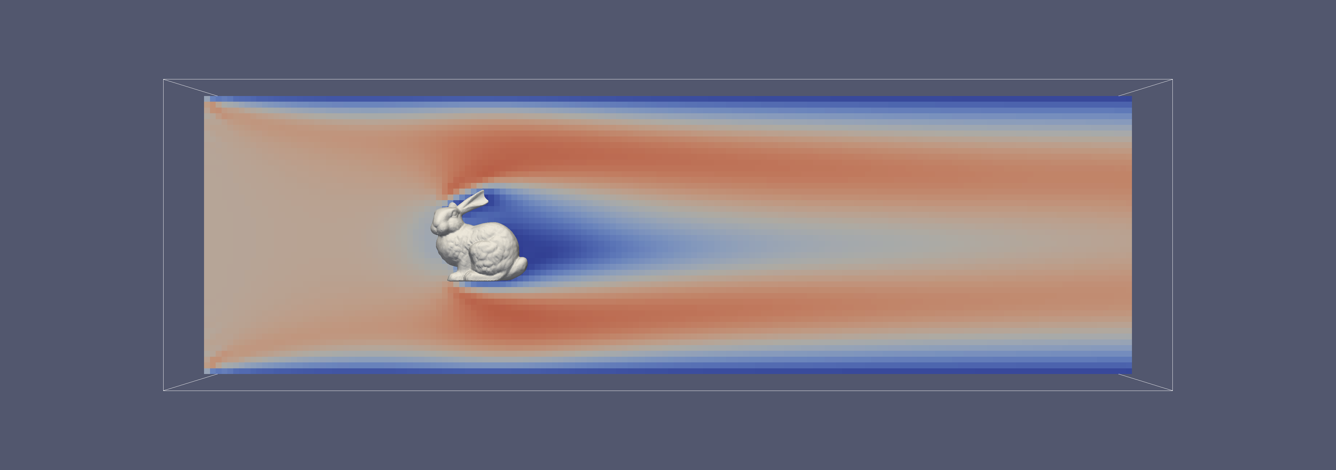
In this application, we will again simulate a channel flow around an obstacle. As before, the application will be fully configurable by a configuration file.

Lattice Boltzmann Data Structures

Lattice Model

In this tutorial, we will use the standard D3Q27 stencil with a SRT collision model.

using LatticeModel_T         = lbm::D3Q27< lbm::collision_model::SRT >;
using Stencil_T              = LatticeModel_T::Stencil;
using CommunicationStencil_T = LatticeModel_T::CommunicationStencil;

As this is only the basic LBM setup, other stencils and collision methods can be included to simulate more accurate, stable and complex flows.

Mesh and Domain

When building waLBerla with the CMAKE configuration WALBERLA_BUILD_WITH_OPENMESH enabled, one can use its capabilities for loading, storing and manipulating meshes. OpenMesh supports many common mesh data formats. We will use an .obj file.

NOTE: with the functions used in this tutorial, only triangle meshes are processed correctly. For more information, please refer to the walberla::mesh module.

Reading meshes into waLBerla is relatively straightforward, even for large scale simulations. Firstly, we define a block in our parameter file responsible for the mesh and the domain:

DomainSetup
{
   meshFile         bunny.obj;
   numLevels        0;
   domainScaling    <  10,  3,  1 >;
   dx               3;
   cellsPerBlock    < 16, 16, 16 >;
   periodic         <  0,  0,  1 >;
}

We will comment on the meaning behind these parameters when they are first used in the code snippets.

The name of the file in which our mesh is stored (here: bunny.obj as we want to simulate a flow around the Stanford Bunny) is parsed as usual:

   // read domain parameters
   auto domainParameters = walberlaEnv.config()->getOneBlock("DomainSetup");
 
   std::string meshFile = domainParameters.getParameter< std::string >("meshFile");

Afterwards, the mesh is read in on a single process and broadcasted to all other processes with

   // read in mesh with vertex colors on a single process and broadcast it
   auto mesh = make_shared< mesh::TriangleMesh >();
   mesh->request_vertex_colors();
   mesh::readAndBroadcast(meshFile, *mesh);

Note that we have requested vertex colors from the mesh for the purpose of coloring the faces of the object according to its vertices in the next step. Therefore we define a helper function vertexToFaceColor that iterates over all faces and colors them in their vertex color. If no uniform coloring of the vertices is given, a default color is taken.

template< typename MeshType >
void vertexToFaceColor(MeshType& mesh, const typename MeshType::Color& defaultColor)
{
   WALBERLA_CHECK(mesh.has_vertex_colors())
   mesh.request_face_colors();
 
   for (auto faceIt = mesh.faces_begin(); faceIt != mesh.faces_end(); ++faceIt)
   {
      typename MeshType::Color vertexColor;
 
      bool useVertexColor = true;
 
      auto vertexIt = mesh.fv_iter(*faceIt);
      WALBERLA_ASSERT(vertexIt.is_valid())
 
      vertexColor = mesh.color(*vertexIt);
 
      ++vertexIt;
      while (vertexIt.is_valid() && useVertexColor)
      {
         if (vertexColor != mesh.color(*vertexIt)) useVertexColor = false;
         ++vertexIt;
      }
 
      mesh.set_color(*faceIt, useVertexColor ? vertexColor : defaultColor);
   }
}

After calling this function, we prepare for building the distance octree by precalculating information (e.g. face normals) of the mesh that is required for computing the singed distances from a point to a triangle:

   // add information to mesh that is required for computing signed distances from a point to a triangle
   auto triDist = make_shared< mesh::TriangleDistance< mesh::TriangleMesh > >(mesh);

From this information we can finally build the distance octree. It stores information about how close or far boundaries are to each other. Later, this information could be used for e.g. adaptive mesh refinement (note that this will not be covered in this tutorial).

   // building distance octree
   auto distanceOctree = make_shared< mesh::DistanceOctree< mesh::TriangleMesh > >(triDist);

When writing the distance octree to disk (e.g. for debugging purposes), care must be taken to execute the write function only on the root node:

   // write distance octree to file
   WALBERLA_ROOT_SECTION()
   {
      distanceOctree->writeVTKOutput("distanceOctree");
   }

Even though we have successfully loaded the complex geometry and set up the corresponding distance octree, we have not defined our computational LB domain yet. In this tutorial, the LB domain is defined relatively to the loaded geometry. Henceforth, we calculate the axis-aligned bounding box of the geometry and scale it to our needs. Here, we chose our channel to be 10x3x1 times the size of the Stanford Bunny. This scaling is defined in the parameter file (parameter: domainScaling). As the bunny will be placed in the center of the bounding box, we shift the center to the left such that the bunny will be nearer to the inflow.

   auto aabb = computeAABB(*mesh);
   aabb.scale(domainScaling);
   aabb.setCenter(aabb.center() + 0.2 * Vector3< real_t >(aabb.xSize(), 0, 0));

Finally, we use a convenient built-in data structure that will be responsible for the creation of the structured block forest and set the periodicity according to the parameter file.

   // create and configure block forest creator
   mesh::ComplexGeometryStructuredBlockforestCreator bfc(aabb, Vector3< real_t >(dx),
                                                         mesh::makeExcludeMeshInterior(distanceOctree, dx));
 
   bfc.setPeriodicity(periodicity);

The ComplexGeometryStructuredBlockforestCreator takes as arguments the axis-aligned bounding box of the domain, the cell sizes dx and an exclusion function. In this tutorial, we want to exclude the interior of the Stanford Bunny with a maximum error of dx. Afterwards, we create the structured block forest on which the sweeps will be performed

   // create block forest
   auto blocks = bfc.createStructuredBlockForest(cellsPerBlock);

Boundary Handling

The rest of the tutorial mainly follows Tutorial 01 and should therefore be self-explanatory. The only adaption that has to be made is the treatment of the boundaries. Whereas the boundary conditions of the basic domain (inflow, outflow, no-slip) can be again treated by the lbm::DefaultBoundaryHandlingFactory, the no-slip boundary conditions of the bunny need special attention. After the standard routine of the lbm::DefaultBoundaryHandlingFactory

   // create and initialize boundary handling
   const FlagUID fluidFlagUID("Fluid");
 
   auto boundariesConfig = walberlaEnv.config()->getOneBlock("Boundaries");
 
   typedef lbm::DefaultBoundaryHandlingFactory< LatticeModel_T, FlagField_T > BHFactory;
 
   BlockDataID boundaryHandlingId = BHFactory::addBoundaryHandlingToStorage(
      blocks, "boundary handling", flagFieldId, pdfFieldId, fluidFlagUID,
      boundariesConfig.getParameter< Vector3< real_t > >("velocity0", Vector3< real_t >()),
      boundariesConfig.getParameter< Vector3< real_t > >("velocity1", Vector3< real_t >()),
      boundariesConfig.getParameter< real_t >("pressure0", real_c(1.0)),
      boundariesConfig.getParameter< real_t >("pressure1", real_c(1.0)));
 

we address the complex geometry. In a first step, the boundaries that we colored in vertexToFaceColor are equipped with the no-slip boundary UID and the boundary information is added to the mesh.

   // set NoSlip UID to boundaries that we colored
   mesh::ColorToBoundaryMapper< mesh::TriangleMesh > colorToBoundaryMapper(
      (mesh::BoundaryInfo(BHFactory::getNoSlipBoundaryUID())));
   colorToBoundaryMapper.set(mesh::TriangleMesh::Color(255, 255, 255),
                             mesh::BoundaryInfo(BHFactory::getNoSlipBoundaryUID()));
 
   // mark boundaries
   auto boundaryLocations = colorToBoundaryMapper.addBoundaryInfoToMesh(*mesh);

In order to have the mesh information available at postprocessing, we write this information to a VTK file as

   // write mesh info to file
   mesh::VTKMeshWriter< mesh::TriangleMesh > meshWriter(mesh, "meshBoundaries", 1);
   meshWriter.addDataSource(make_shared< mesh::BoundaryUIDFaceDataSource< mesh::TriangleMesh > >(boundaryLocations));
   meshWriter.addDataSource(make_shared< mesh::ColorFaceDataSource< mesh::TriangleMesh > >());
   meshWriter.addDataSource(make_shared< mesh::ColorVertexDataSource< mesh::TriangleMesh > >());
   meshWriter();

Lastly, the boundary information of the complex geometry is added to the structured block forest and the fluid cells and the boundaries are set accordingly.

   // voxelize mesh
   mesh::BoundarySetup boundarySetup(blocks, makeMeshDistanceFunction(distanceOctree), numGhostLayers);
 
   // set fluid cells
   boundarySetup.setDomainCells< BHFactory::BoundaryHandling >(boundaryHandlingId, mesh::BoundarySetup::OUTSIDE);
 
   // set up inflow/outflow/wall boundaries from DefaultBoundaryHandlingFactory
   geometry::initBoundaryHandling< BHFactory::BoundaryHandling >(*blocks, boundaryHandlingId, boundariesConfig);
   // set up obstacle boundaries from file
   boundarySetup.setBoundaries< BHFactory::BoundaryHandling >(
      boundaryHandlingId, makeBoundaryLocationFunction(distanceOctree, boundaryLocations), mesh::BoundarySetup::INSIDE);

Outlook

Now that you have seen how to load and process complex geometries from a mesh file, you can play around with this tutorial and adapt it to your needs.

Suggestions for further improvement are the already mentioned adaptive refinement of the loaded geometry. Load balancing of the resulting blocks is then recommended. Thin can be done by using functionalities of mesh::ComplexGeometryStructuredBlockforestCreator and mesh::MeshWorkloadMemory, respectively.