A configurable application for simulation of backward-facing step problem

Overview

The aim of this tutorial is to show how to build and solve the backward-facing step model using lattice Boltzmann method in waLBerla. The "01_BasicLBM" case is used as the foundation of the current work. Therefore, most of the functionalities have already been introduced and discussed in LBM 1 tutorial. Here the main focus is on the following areas:

parameterization with the help of the Reynolds number
setting up the step geometry with the help of the input file
evaluation of the recirculation length

Backward-facing step (implemented by a box shape in configuration file) in a 2D channel, Re=400

General Setup

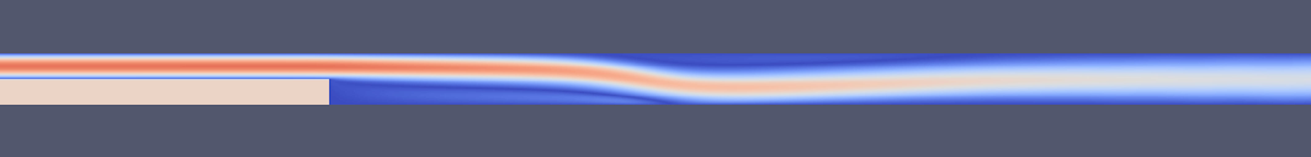
A 2D channel flow with a backward-facing step is simulated. The application is configured with the Reynolds number and lattice velocity as input and reattachment location as the output. The input parameters are specified in a configuration file while the calculation and writing of reattachment locations are performed in a functor ReattachmentLengthFinder which is implemented inside the program.

Lattice Boltzmann Model

Since the simulations are carried out in 2D, the standard D2Q9 stencil with SRT collision model is used which is already implemented in the 'lbm' module.

using LatticeModel_T = lbm::D2Q9<lbm::collision_model::SRT>;
using Stencil_T = LatticeModel_T::Stencil;
using CommunicationStencil_T = LatticeModel_T::CommunicationStencil;

Parameterization with Reynolds number

The main() function must be modified so that the program could accept the Reynolds number and lattice velocity as input parameters. These parameters are specified in the 'parameters' section of the config file.

Parameters 
{
    Re              400;
    timesteps       10000000;
    uLB             0.05;
    remainingTimeLoggerFrequency 3; // in seconds
    loggingFrequency 50; // in time steps
}

The following lines inside the main() function reads these two values from the parameters section of the configuration file:

const real_t Re = parameters.getParameter< real_t >( "Re", real_c( 1000 ) );

const real_t uLB = parameters.getParameter< real_t >( "uLB", real_c( 0.01 ) );

The height of the channel is considered as the reference length in this simulation (it may differ in other applications). This value is read from the DomainSetup section in the configuration file where the dimensions of the channel are specified.

const Vector3<real_t> domainsize = domain.getParameter< Vector3<real_t> >( "cellsPerBlock", Vector3<real_t>() );

Finally, viscosity consequently omega are calculated with the Reynolds number, lattice velocity and reference length.

const real_t viscosity = (domainsize[1] * uLB) / Re;

const real_t omega = lbm::collision_model::omegaFromViscosity(viscosity);

Geometry

Since the step geometry is a plain rectangular area, the simplest approach is to create it by geometry module in walberla. This module offers capability to read boundaries of a random geometry from images, voxel files, coordinates of vertices, etc. Using this module, obstacles of basic shapes could be conveniently positioned inside the domain. It is also easier to have the program to read the geometry specifications from the Boundaries section of the configuration file. This is implemented by reading and storing the Boundaries block of the configuration file in 'boundariesConfig' object and passing it to a convenience function provided in the geometry class to initialize the boundaries.

geometry::initBoundaryHandling<BHFactory::BoundaryHandling>( *blocks, boundaryHandlingID, boundariesConfig );

Here a subblock 'Body' is created inside 'Boundaries' section in the configuration file in order to create a box (rectangle in 2D) using two diagonal vertices.

    Body
    {
       shape box;
       min <0,0,0>;
       max <2000,50,1>;
       NoSlip {} 
    }

For more details about specifying boundaries using configuration file, please refer to the documentation of walberla::geometry::initBoundaryHandling().

Evaluation of the recirculation length

In order to find the reattachment location precisely, the velocity on each lattice cell on the bottom boundary line of the domain following the step is examined. The idea is to locate the exact position on the bottom boundary in which the streamwise velocity component switches sign. This mechanism is implemented by a functor named ReattachmentLengthFinder and is passed to a method of timeloop 'addFuncBeforeTimeStep()'' to create the logger.

   std::string loggingFileName = "ReattachmentLengthLogging_Re" + std::to_string(uint_c(Re)) + ".txt";
   uint_t loggingFrequency = parameters.getParameter< uint_t >( "loggingFrequency", uint_c(1) );
   Vector3<real_t> stepSize = boundariesConfig.getOneBlock("Body").getParameter< Vector3<real_t> >("max", Vector3<real_t>() );
 
   timeloop.addFuncAfterTimeStep( ReattachmentLengthFinder( blocks, pdfFieldID, flagFieldID, fluidFlagUID,
                                                            loggingFileName, loggingFrequency, stepSize ),
                                  "reattachment length finder" );

After running the program, the locations of reattachment against timestep are written to 'ReattachmentLengthLogging_Re_[Re].txt' in the working directory. Note that there might be more than one reattachment location before the flow fully develops along the channel, and all are given in the file. This simply means that it is expected to have multiple occurences of seperation and reattachment at the same time along the bottom boundary of the channel following the step in the early stages. However, most of them are smeared later as the flow starts to develop. The logging frequency can also be adjusted by 'checkFrequency' which is passed to the ReattachmentLengthFinder functor.

Results

The following results of the normalized reattachment length were obtained by a numerical study, using the here developed application. Note that it might take a long time until the simulation has reached a steady state and the final values for this length can be obtained. Also, the step has to be long enough to feature a converged, parabolic flow profile before the expansion, and the domain itself has to be long enough to not perturb the results by the vicinity of the outflow boundary condition. Reference results were taken from Ercan Erturk, “Numerical solutions of 2-D steady incompressible flow over a backward-facing step, Part I: High Reynolds number solutions”, Computers & Fluids, Vol. 37, 2008.

Normalized recirculation length for different Re
Re	simulation	literature	% of difference
100	2.880	2.922	1.44
200	4.940	4.982	0.84
300	6.700	6.751	0.76
400	8.180	8.237	0.69
500	9.360	9.420	0.64
600	10.300	10.349	0.47
700	11.080	11.129	0.44
800	11.780	11.834	0.46
900	12.420	12.494	0.59
1000	13.040	13.121	0.62

Outlook

To improve this application, parallelization with a proper synchronization of the reattachment lengths could be added. Also, a stopping criterion based on the convergence of some relevant quantity could be added to avoid a manual termination of the simulation.

Table of Contents