 |
waLBerla 7.2
|
|
waLBerla 7.2
|
Unsteady heat equation, implicit time stepping, VTK output and ParaView, parallelization with MPI, residual based termination. File 06_HeatEquation.cpp.
In this tutorial, we will make use of the Jacobi method implemented in Tutorial - PDE 1: Solving PDEs with the Jacobi Method to solve the linear system of equations that arises by the implicit time discretization of the unsteady heat equation. The implementation is further improved by using VTK output, parallelization with MPI, and a residual based termination of the Jacobi iteration.
The heat equation is a classical example for a parabolic partial differential equation, given by:
\[ \frac{\partial u(x,y,t)}{\partial t} = \kappa \left( \frac{\partial^2 u(x,y,t)}{\partial x^2} + \frac{\partial^2 u(x,y,t)}{\partial y^2}\right) \]
It includes the unknown \(u(x,y,t)\) which can be any scalar, and often is regarded physically as the temperature, and the thermal diffusivity \(\kappa\). In our case, the domain is \(\Omega=[0,1]\times[0,1]\), the Dirichlet boundary conditions are zero everywhere, and the initial distribution of \(u\) inside the domain is given by the initial condition
\[ u(x,y,0) = \sin(\pi x) \sin(\pi y). \]
For the numerical solution, we not only have to discretize in space but also in time. The latter is done via an implicit Euler method with a time step \(\Delta t\), resulting in the following formulation:
\[ \frac{u^{new} - u^{old}}{\Delta t} = \kappa \left( \frac{\partial^2 u^{new}}{\partial x^2} + \frac{\partial^2 u^{new}}{\partial y^2}\right) \]
So in contrast to an explicit Euler method, where the values on the right-hand side would be of the old time step, resulting in a simple update step, we have to solve a system of equations in each time step.
Together with the finite-difference spatial discretization, introduced in the previous tutorial, this leads to:
\[ u_{i,j}^{new} - \kappa\,\Delta t\left[\frac{1}{(\Delta x)^2} \left(u_{i+1,j}^{new} - 2u_{i,j}^{new} + u_{i-1,j}^{new}\right) + \frac{1}{(\Delta y)^2} \left(u_{i,j+1}^{new} - 2u_{i,j}^{new} + u_{i,j-1}^{new}\right)\right] = u_{i,j}^{old} \]
Upon closer inspection, you will notice that this equation looks very similar to the one we had obtained by discretizing the elliptic PDE in the previous tutorial. In fact, the overall structure is exactly the same, i.e., speaking in stencils we again have a D2Q5 stencil, only the weights of the different contributions have slightly changed. Thus, our Jacobi method can again be used to solve this system arising in each time step. The iteration formula for the Jacobi method is given as:
\[ u_{i,j}^{new,(n+1)} = \left(\frac{2\kappa\,\Delta t}{(\Delta x)^2} + \frac{2 \kappa\,\Delta t}{(\Delta y)^2} + 1\right)^{-1} \left[\frac{\kappa\,\Delta t}{(\Delta x)^2} \left(u_{i+1,j}^{new,(n)} + u_{i-1,j}^{new,(n)}\right) + \frac{\kappa\,\Delta t}{(\Delta y)^2} \left(u_{i,j+1}^{new,(n)} + u_{i,j-1}^{new,(n)}\right) + u_{i,j}^{old}\right] \]
Before moving on, let's take a moment to clarify the differences to the previous tutorial as they are essential to understand the next steps. As you can see from the superscripts of \( u \), we now have actually two loops:
The important fact is that in waLBerla it is not possible to incorporate one time loop object into another one to resemble the two loops. Therefore, a slight change in the program structure is necessary. We will implement the entire Jacobi iteration procedure in the JacobiIteration class. This functor includes all the steps that were carried out before by the time loop object, i.e., iterating a specified number of times, calling the communication routine to update the ghost layers of the blocks, and executing the Jacobi sweep. So, no new functionality has to be added but only the structure of the program is adapted. The private members of this class are
These three additional members are needed to carry out the former tasks of the time loop. The implementation reads as:
As you can see, the innermost part is the former Jacobi sweep from the JacobiSweepStencil class. It is enclosed by the loop over all blocks, just like it was done in the initBC() and initRHS() functions from before. Before this iteration can be carried out, the ghost layer cells have to be updated, achieved by the myCommScheme_() call. The iterations, that were done by the time loop object, are now done explicitly with the loop over i until the maximum number of iterations is reached.
This functor is now registered at the time loop object via:
The Jacobi method expects the old solution as the right-hand side function. This means that in each time step, before calling the Jacobi method, the old solution, which is present in the src field, has to be transferred to the rhs field. There are many possibilities to do this. Here, we implement a small class Reinitialize, which simply swaps the src and rhs pointers.
On a side note, this means that the starting solution for the Jacobi method is the former right-hand side. This is more advantageous compared to setting it always to zero (which could be done via src->set( real_c(0) )) as it is probably already quite close to the converged solution, i.e., the Jacobi method will converge faster.
This functor is now registered as a sweep in the time loop in the known fashion:
It is now left to initialize the src field with the initial condition \(u(x,y,0)\). This is similar to what was done in the previous tutorial for the right-hand side function \(f\).
With this, all parts are present and the simulation can be started.
No worries, everything we did was correct but the color gets automatically scaled in each time step. Since the initial profile just shrinks over time, the results will always look the same. When you use the numeric representation, you will actually see changes in the values, which get smaller from one time step to the next one.
This brings us to three additional points that will be covered in the remainder of this tutorial:
You find all those extensions in the file 06_HeatEquation_Extensions.cpp.
Making our code write VTK files as output is actually very easy thanks to already available functions. Here is what we have to add:
The createVTKOutput function has two templates, specifying the type of field we want to write, here ScalarField, and of which data type this output shall be. Here we explicitly state float as this is usually accurate enough for data analysis purposes and saves disk space/IO bandwidth. As arguments, the field we want to output together with the block structure and a name for the data has to be given. The fourth argument specifies the write frequency where the value 1 denotes that we want to have an output after every time step. The number of ghost layers that are written can be specified by the fifth argument, where in our case we only have one and output it.
To start the simulation, we simply write:
This creates a folder vtk_out, including a solution.pvd file and a folder solution that actually includes the output of the different time steps.
Now we start ParaView and open the solution.pvd file.
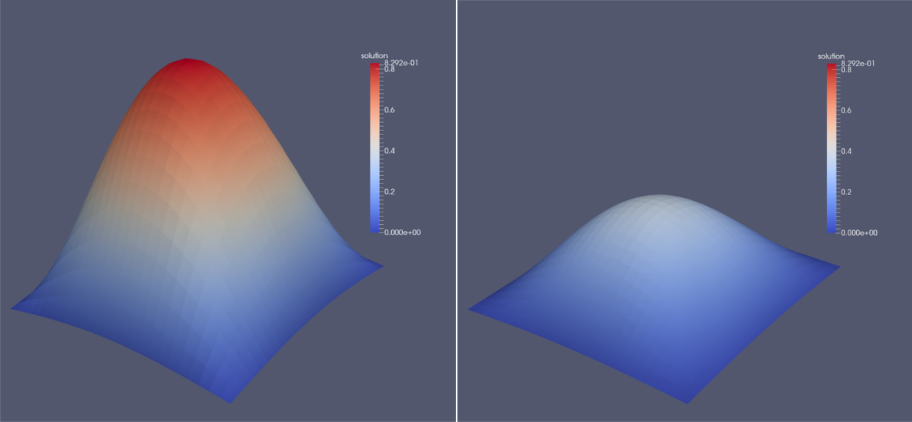
This file manages all the files from the solution folder and makes them available in ParaView. Additionally, if multiple blocks were used, ParaView will automatically merge them so we can inspect the whole domain. Since ParaView knows the concept of ghost layers which surround the whole domain but are not displayed by default, no data can be seen at first. We first have to use a Slice filter with the normal in z-direction. Apart from the surface representation of the solution field, it is possible to generate a three dimensional visualization of this scalar field. To do so, the filters Cell Data to Point Data and Warp By Scalar have to be applied consecutively. The image below shows an exemplary solution after the first and fifth time step.
As you may have noticed, the simulation already takes quite some time to finish. For larger problems, running the simulation with multiple processes is often advantageous or even absolutely necessary. Since waLBerla is developed with a special focus on high performance computing, the parallelization feature is included and can easily be used. We have seen the implications of this functionality before:
Since we have already applied these concepts, the changes to the code boil down to one thing: The first boolean flag given to the blockforest::createUniformBlockGrid function has to be set to true. This will assign each block to exactly one process, i.e., we have to use as many blocks as we have processes. Suppose we want to run the program with 4 processes, we could use two blocks in x- and y-direction, respectively.
Then we run the program with the command mpirun -np 4 ./06_HeatEquation_Extensions.
To prohibit a false usage of the program, we can include an if statement at the beginning of the program. It checks if the number of used processes is in fact equal to the number of blocks and ends the program if not.
If you visualize the data in ParaView with the Warp By Scalar functionality, you will see a strange hole in the center of the domain. This is due to the fact that ParaView uses the information inside the ghost layers for the visualization (but does not display them explicitly). Those ghost layers, however, still have the value 0 right at the corner at the domain center since the D2Q5 stencil does not need those values and thus the communication scheme does not need to update it. This can be fixed by setting up an additional communication scheme with a D2Q9 stencil and calling this function right before the VTK output is written. Run the program with this additional communication step and check the results.
One last very common feature is still missing. Iterative solvers are usually terminated when the solution is sufficiently converged. One measure of convergence is the norm of the residual \( r = b-\textbf{A}x\), that has to drop below a specific threshold. A suitable norm is the weighted L2-norm, which accounts for the number of cells ( \(N\)) inside the domain:
\[ \| r \| = \sqrt{ \frac{1}{N} \sum_{i=0}^{N-1} r_i^2} \]
The computation of this residual might look straight-forward: We simply apply the stencil to each cell, add up these values, and subtract it from the right hand side. The difficulty arises because of the sum over ALL cells inside the domain. With multiple blocks present, the local block-sums thus have to be shared with all other blocks (on other processes) and summed up. Additionally, every process has to know the total number of cells inside the domain to be able to divide by \(N\). Only then, the square root can be calculated and the norm of the residual can be obtained.
These two peculiarities are accomplished with the function mpi::allReduceInplace that does exactly this: gather the local sum values of all processes, combine them by, in our case, summing them up, and communicate the result to all processes again.
Our implementation is thus extended by two additional functions, yielding the JacobiIterationResidual class. The one that computes the total number of cells inside the domain and stores it in the private member cells_ is implemented as:
The actual computation of the residual is then:
The termination of the Jacobi iteration is then accomplished by introducing a check after the Jacobi sweep, which makes use of the private member residualThreshold_ :
The WALBERLA_ROOT_SECTION is a special macro that ensures that the content is only executed by one process, namely the root process. Otherwise, this output would appear multiple times when running in parallel. Feel free to test it.
Solving linear systems of equations is a very common task in various applications. Thus, waLBerla already provides ready-to-use implementations of some iterative solvers: Jacobi method, Red-Black Gauss-Seidel method, and Conjugate gradients. You find the implementations in the src/pde/ folder and how to use them is shown in the test cases under src/tests/pde/. Even the more involved CG method can be implemented with the concepts we developed until now.